PostgreSQL EXPLAIN ANALYZE For Real Queries

You've written the query. It works. It returns the right rows.

It's also slow.

You add an index. It's still slow. You add another index. Now it's slower. You stare at the query for ten minutes, convinced there must be a missing WHERE. There isn't. The query is fine. The plan isn't.

This is the part where most people learn that EXPLAIN ANALYZE exists, run it, see a wall of indented text, and quietly close the terminal.

Let's not do that. The output looks intimidating, but every number on the page means something specific, and once you've read fifty plans you'll see the patterns the same way an experienced SRE reads a flame graph. The trick is knowing which numbers actually matter and which ones are decoration.

This piece walks through what EXPLAIN ANALYZE shows you, what each metric is really telling you, and the small handful of patterns that catch most slow queries in the wild. Real plans, real numbers, real interpretation.

EXPLAIN vs EXPLAIN ANALYZE, they're not the same

EXPLAIN shows the plan the planner would use, with estimates. Nothing executes. It's fast, it's safe, and the numbers are guesses based on table statistics.

EXPLAIN ANALYZE actually runs the query and shows what happened. The plan is annotated with real timings, real row counts, and (if you ask for it) real buffer reads.

-- Just the estimated plan, no execution
EXPLAIN SELECT * FROM orders WHERE status = 'pending';

-- Actually runs the query and reports what happened
EXPLAIN ANALYZE SELECT * FROM orders WHERE status = 'pending';

-- The version you almost always want in practice
EXPLAIN (ANALYZE, BUFFERS) SELECT * FROM orders WHERE status = 'pending';

Two things to remember before you reach for ANALYZE:

It runs the query. If your query is DELETE FROM orders or an UPDATE that locks half the table, EXPLAIN ANALYZE will execute it. Wrap mutations in a transaction you intend to roll back:

BEGIN;
EXPLAIN (ANALYZE, BUFFERS) UPDATE orders SET status = 'archived' WHERE created_at < '2020-01-01';
ROLLBACK;

BUFFERS is the metric most people skip and shouldn't. It's the difference between a query that's slow because it's doing real I/O and a query that's slow because it's doing pointless work in cache. Always ask for it.

How to read a plan tree

A plan is a tree. The root at the top is the final result. Indented children below are the inputs that feed it. Postgres reads bottom-up; you read it bottom-up too.

Take this query against an orders table with a few hundred thousand rows:

EXPLAIN (ANALYZE, BUFFERS)
SELECT customer_id, COUNT(*)
FROM orders
WHERE status = 'pending'
GROUP BY customer_id;

A typical plan might look like this:

HashAggregate  (cost=4523.10..4612.45 rows=8935 width=12)
               (actual time=42.118..43.902 rows=9120 loops=1)
  Group Key: customer_id
  Buffers: shared hit=1843
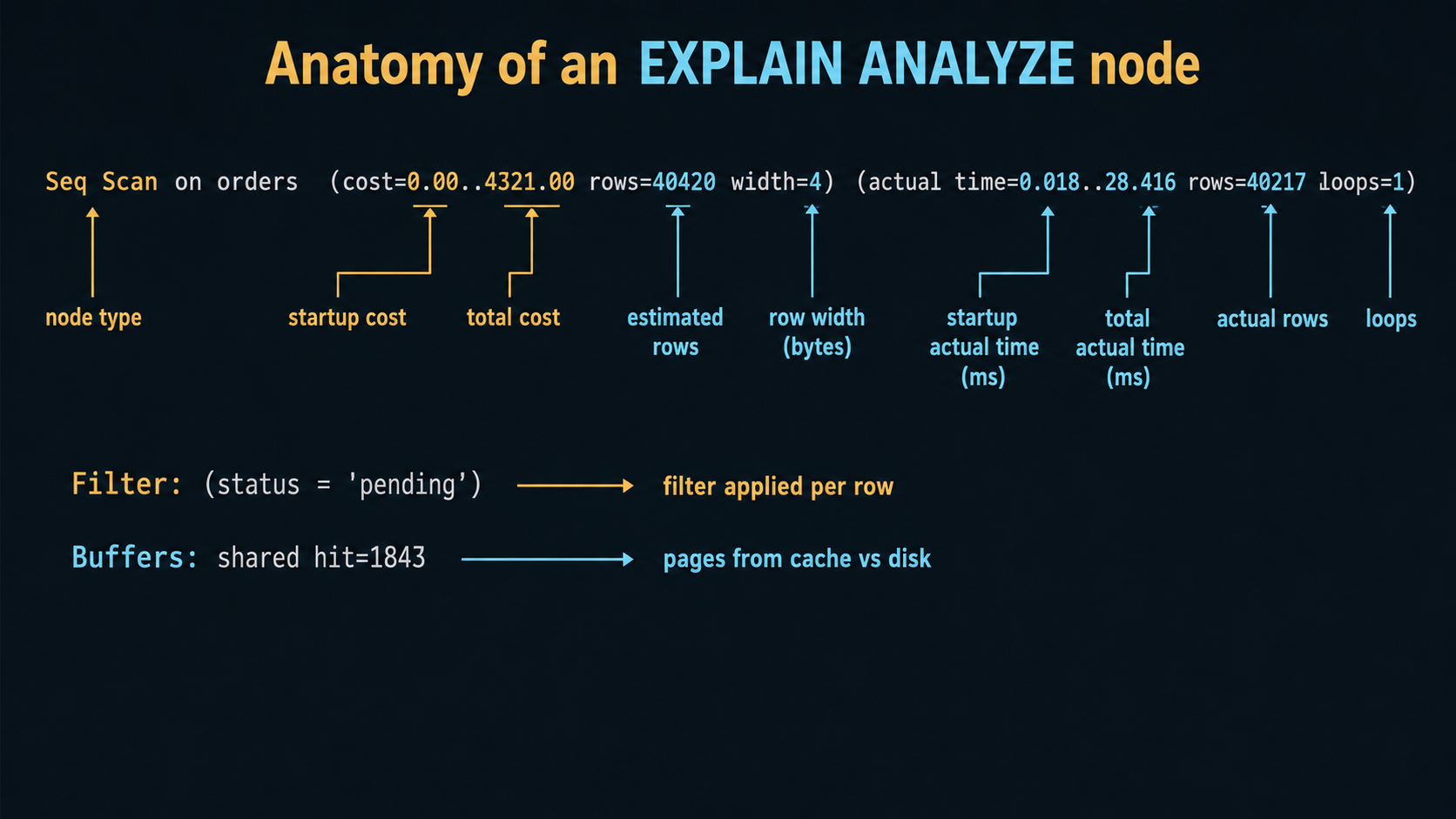
  ->  Seq Scan on orders  (cost=0.00..4321.00 rows=40420 width=4)
                          (actual time=0.018..28.416 rows=40217 loops=1)
        Filter: (status = 'pending')
        Rows Removed by Filter: 159783
        Buffers: shared hit=1843
Planning Time: 0.214 ms
Execution Time: 44.512 ms

The bottom node, Seq Scan on orders, runs first. It scans the whole table, applies the WHERE filter, and produces 40,217 rows. That feeds HashAggregate, which buckets those rows by customer_id and counts. The arrow -> is "this feeds the parent above me."

Every node has the same anatomy. Once you can read one node, you can read any plan, no matter how scary the indentation looks.

Cost, what the planner believes

The first parenthetical, (cost=0.00..4321.00 rows=40420 width=4), is what the planner estimated before running anything.

The two numbers are startup cost and total cost. Startup is the work done before the first row can be returned; total is the work done to return the last row. For a Seq Scan startup is essentially zero, because you start streaming rows immediately. For a Sort, startup equals total because you can't return any sorted row until you've seen every input row.

The unit is "cost units," not milliseconds. They're calibrated against seq_page_cost (default 1.0), random_page_cost (default 4.0), and the various *_op_cost settings. A cost of 4321 doesn't mean 4321 of anything you can hold in your hand. It means "this much work" in the planner's internal accounting.

Cost matters for one thing: comparing alternatives. The planner picks the lowest-cost plan it can find. If you suspect the wrong plan was chosen, comparing costs tells you whether the planner thought its choice was cheaper. If the chosen plan has cost 4000 and the index scan you wanted has cost 12000, the planner isn't broken. It genuinely believed the seq scan was cheaper. Your job then is to figure out why the planner believed that, which usually leads back to statistics.

rows=40420 is the planner's estimate of how many rows this node will produce. width=4 is the average row width in bytes, useful when you're worried about memory for sorts and hashes, mostly noise otherwise.

Actual time and actual rows, what really happened

The second parenthetical, (actual time=0.018..28.416 rows=40217 loops=1), is what ANALYZE measured.

actual time=0.018..28.416 is startup..total in milliseconds, like cost but real. The first value is the time until the first row was emitted; the second is the time until the last row was emitted. For nodes that have to consume their entire input before emitting anything (Sort, HashAggregate, Hash), startup will be close to total.

rows=40217 is the actual number of rows produced, not estimated. This is the most diagnostic number on the entire page. Compare it to the estimate above.

loops=1 is critical and almost always misread. The actual time and actual rows are reported per loop, not totals. If loops=1, fine, those are the totals. If loops=2500, you have to multiply.

Here's a plan fragment where this matters:

Nested Loop  (cost=0.42..18234.10 rows=2500 width=80)
             (actual time=0.045..2812.301 rows=2487 loops=1)
  ->  Index Scan using orders_status_idx on orders  (rows=2500 loops=1)
        (actual time=0.022..14.301 rows=2487 loops=1)
  ->  Index Scan using customers_pkey on customers  (rows=1 loops=2487)
        (actual time=1.118..1.121 rows=1 loops=2487)

That last node looks innocent: 1.12 ms per execution, one row per execution. But loops=2487. Total time spent in that node is roughly 1.121 * 2487 ≈ 2787 ms. The Nested Loop's total actual time=...2812.301 matches that. The slowness isn't the outer scan; it's the 2487 round-trips through the inner index. That's a Nested Loop that probably wants to be a Hash Join.

When you read a plan, watch for nodes with high loops and any per-loop cost above ~0.5 ms. Multiplied out, that's where the time goes.

Estimated rows vs actual rows, the smoking gun

The single most useful exercise in plan reading is comparing the planner's row estimate to the actual row count, top to bottom. Big mismatches are why bad plans happen.

Look at this fragment:

Hash Join  (cost=823.00..2104.50 rows=1 width=124)
           (actual time=12.418..318.207 rows=84510 loops=1)

The planner thought this join would produce 1 row. It actually produced 84,510 rows. The planner picked a Hash Join based on the assumption that the result would be tiny. Now imagine the next node up the tree is a Nested Loop that uses this output as its outer side. The planner thought it'd loop once. It will loop 84,510 times.

That's how a query goes from 50 ms to 50 seconds. Not because Postgres is broken. Because the statistics lied, and a chain of decisions downstream were all built on the lie.

A rule of thumb: ratios under 10x are usually fine, ratios above 100x are worth investigating, ratios above 1000x are almost always the cause of whatever pain you're feeling. When you spot one, ask:

Is the column missing from pg_stats? ANALYZE tablename rebuilds statistics. If statistics are wildly stale, the planner is flying blind:

ANALYZE orders;
SELECT attname, n_distinct, most_common_vals
FROM pg_stats
WHERE tablename = 'orders' AND attname = 'status';

Is the data skewed? status = 'pending' might match 0.1% of rows in dev and 40% in production. The planner doesn't know your traffic shape; it knows histograms. Bumping default_statistics_target for a specific column gives the planner a finer-grained picture:

ALTER TABLE orders ALTER COLUMN status SET STATISTICS 1000;
ANALYZE orders;

Are correlated columns being treated as independent? The planner assumes column predicates multiply: WHERE country = 'US' AND state = 'CA' is treated as P(country=US) * P(state=CA), which dramatically underestimates because state implies country. Extended statistics fix this:

CREATE STATISTICS orders_country_state (dependencies)
  ON country, state FROM orders;
ANALYZE orders;

The estimate-vs-actual gap is the closest thing Postgres has to a "this is why your query is slow" indicator. Train your eye on it.

Buffers, what was actually read

Add BUFFERS to your EXPLAIN ANALYZE and you'll see lines like:

Buffers: shared hit=43210 read=1284 dirtied=12 written=0

These count 8 KB pages, not bytes or rows.

shared covers pages from regular tables and their indexes. hit is "found in the buffer cache, no disk I/O." read is "had to fetch from disk (or OS cache)." dirtied is "this query modified the page." written is "had to flush a dirty page during execution to make room."

There's also local for temp tables and temp for hash/sort spills, and that last one is important. If you see temp read=... it means the query exceeded work_mem and spilled to disk, which is almost always slower than you want.

Two practical heuristics:

Same buffer count, different times. If a query is sometimes 200 ms and sometimes 4 seconds but the plan and buffer counts are identical, it's a cache effect. The fast run hit warm pages; the slow run hit cold disk. The query itself is fine. Capacity planning isn't.

High read, low hit. Cold cache or working set bigger than shared_buffers. Possible fixes: cover the query with a smaller index (less to read), reduce the rows returned, or accept that disk speed bounds you.

temp written showing up. A sort or hash spilled. If work_mem=4MB and your sort needs 80 MB, you've just spent the query running disk I/O on intermediate results. Either bump work_mem for that session, rewrite to sort less, or add an index that returns rows already-ordered.

Buffers are blind spots in monitoring tools that report execution time only. Two queries can both run in 100 ms, one hitting 50 cached pages, the other hitting 50,000. Under load, the second one falls off a cliff. BUFFERS is how you see that before it happens.

A real query, sequential scan vs index

Let's walk through one. Same query, two plans, one with an index and one without.

SELECT id, customer_id, total
FROM orders
WHERE created_at >= '2022-04-01' AND created_at < '2022-05-01'
ORDER BY created_at DESC
LIMIT 50;

Without an index on created_at:

Limit  (cost=8421.45..8421.58 rows=50 width=24)
       (actual time=187.412..187.428 rows=50 loops=1)
  Buffers: shared hit=1232 read=4521
  ->  Sort  (cost=8421.45..8520.10 rows=39456 width=24)
            (actual time=187.410..187.420 rows=50 loops=1)
        Sort Key: created_at DESC
        Sort Method: top-N heapsort  Memory: 28kB
        Buffers: shared hit=1232 read=4521
        ->  Seq Scan on orders  (cost=0.00..7102.00 rows=39456 width=24)
                                (actual time=0.024..174.501 rows=39812 loops=1)
              Filter: ((created_at >= '2022-04-01') AND (created_at < '2022-05-01'))
              Rows Removed by Filter: 460188
              Buffers: shared hit=1232 read=4521
Planning Time: 0.231 ms
Execution Time: 187.512 ms

Postgres reads the entire orders table (500,000 rows), filters down to ~40,000, sorts them, and returns the top 50. Rows Removed by Filter: 460188 is the planner saying "I threw away 92% of what I read." Buffers: shared read=4521 means roughly 35 MB of disk I/O.

Add an index:

CREATE INDEX orders_created_at_idx ON orders (created_at);
ANALYZE orders;

Re-run the query:

Limit  (cost=0.42..14.81 rows=50 width=24)
       (actual time=0.031..0.412 rows=50 loops=1)
  Buffers: shared hit=54
  ->  Index Scan Backward using orders_created_at_idx on orders
        (cost=0.42..11346.20 rows=39456 width=24)
        (actual time=0.030..0.405 rows=50 loops=1)
        Index Cond: ((created_at >= '2022-04-01') AND (created_at < '2022-05-01'))
        Buffers: shared hit=54
Planning Time: 0.193 ms
Execution Time: 0.452 ms

Three things to notice. The Index Scan Backward walks the index in reverse order, which means the ORDER BY created_at DESC is satisfied by the index, so no separate Sort node. The LIMIT 50 stops the scan after 50 matches because results arrive already-ordered. Buffers dropped from 5,753 to 54, and execution time dropped from 187 ms to 0.5 ms.

This is the canonical case where adding an index pays off enormously: range filter plus order-by plus limit, all aligned on one column. When the order-by isn't aligned with the filter column, you usually want a composite index where the leading columns are the equality filters and the trailing columns are the order-by.

Index Scan, Bitmap Heap Scan, Index Only Scan

Three nodes that all start with "Index" and confuse people who haven't seen them side by side.

Index Scan walks the index, follows each matching entry to the heap (the actual table page), and reads the row. Good for small result sets, because the cost is roughly proportional to rows returned.

Bitmap Index Scan + Bitmap Heap Scan is what Postgres uses when the index would match many rows. It scans the index, builds a bitmap of which heap pages contain matches, then reads each page once and pulls all matching rows. This trades random reads for sequential reads on the heap:

Bitmap Heap Scan on orders  (cost=89.45..1843.20 rows=4500 width=24)
                            (actual time=12.301..38.412 rows=4421 loops=1)
  Recheck Cond: (status = 'pending')
  Heap Blocks: exact=412
  Buffers: shared hit=420
  ->  Bitmap Index Scan on orders_status_idx
        (cost=0.00..88.32 rows=4500 width=0)
        (actual time=11.812..11.812 rows=4421 loops=1)
        Index Cond: (status = 'pending')
        Buffers: shared hit=8

Heap Blocks: exact=412 says the heap was read in 412 page-aligned chunks. Recheck Cond is displayed on every Bitmap Heap Scan, but the recheck only actually executes when the bitmap has lossy pages (Heap Blocks: lossy=N) or the underlying index access method is itself lossy (GiST, GIN). For most btree-driven bitmaps with exact=N and no lossy=, the recheck is a no-op you can ignore.

Index Only Scan is what you want for read-heavy paths. Postgres answers the query entirely from the index without touching the heap:

Index Only Scan using orders_customer_status_idx on orders
  (cost=0.42..18.45 rows=210 width=8)
  (actual time=0.029..0.412 rows=204 loops=1)
  Index Cond: (customer_id = 4231)
  Heap Fetches: 4
  Buffers: shared hit=11

Heap Fetches: 4 is the catch. Even with an Index Only Scan, Postgres still has to check the visibility map to confirm a row is visible to your transaction. If recently-modified pages aren't yet marked all-visible, Postgres falls back to the heap for those rows. Lots of Heap Fetches after a heavy write is normal until autovacuum updates the visibility map. If Heap Fetches stays high indefinitely, autovacuum is falling behind.

For an Index Only Scan to work, every column the query needs must be in the index, including columns in the SELECT list. That's what INCLUDE is for:

CREATE INDEX orders_customer_idx
  ON orders (customer_id)
  INCLUDE (status, total);

customer_id is the indexed key; status and total are stored in the index leaf pages without affecting key ordering. Queries that filter on customer_id and only read status and total get an Index Only Scan for free.

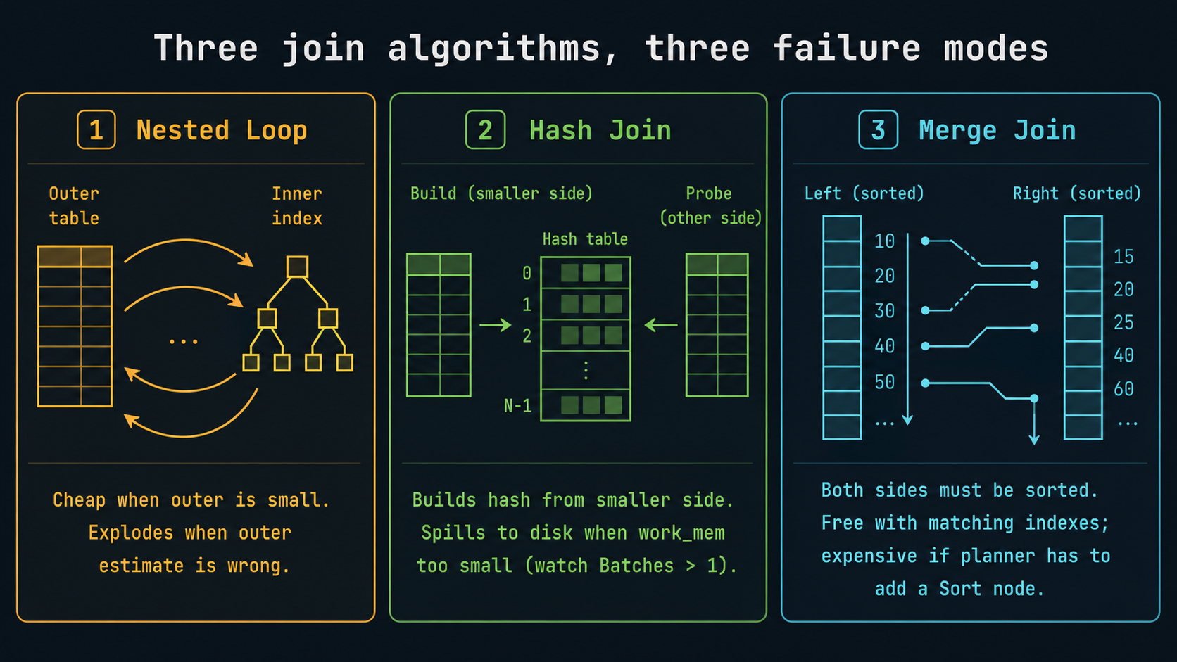
Joins: Nested Loop, Hash Join, Merge Join

Three join algorithms; the planner picks one based on row estimates and available indexes. They each fail in different ways, and the failure mode is usually visible in the plan.

Nested Loop. For each row from the outer side, look up matches on the inner side. Cheap when the outer side is small (think tens to a few thousand rows). Disastrous when the outer side is bigger than the planner expected:

Nested Loop  (cost=0.85..423.10 rows=12 width=80)
             (actual time=0.412..18412.301 rows=84510 loops=1)
  ->  Index Scan on customers  (rows=12) (actual rows=84510 loops=1)
  ->  Index Scan on orders  (rows=1 loops=12) (actual rows=4 loops=84510)

Planner estimated 12 outer rows, got 84,510. Nested Loop ran the inner index scan 84,510 times instead of 12. Total time exploded. Fix the estimate (statistics, extended statistics, query rewrite) and Postgres will likely switch to Hash Join.

Hash Join. Build a hash table from the smaller side, probe it with the larger side. Great when one side fits in work_mem. Look for Memory Usage and Batches:

Hash Join  (cost=423.00..1284.10 rows=84512 width=80)
           (actual time=12.301..118.412 rows=84510 loops=1)
  Hash Cond: (orders.customer_id = customers.id)
  ->  Seq Scan on orders  ...
  ->  Hash  (cost=302.00..302.00 rows=12000 width=72)
            (actual time=11.812..11.812 rows=12000 loops=1)
        Buckets: 16384  Batches: 1  Memory Usage: 1024kB
        ->  Seq Scan on customers  ...

Batches: 1 means the hash fit in memory. Batches: 8 would mean the hash spilled and was rebuilt 8 times, which means work_mem is too small for this query.

Merge Join. Both sides must arrive sorted on the join key. Cheap if both sides are already sorted (typically by index). Otherwise the planner has to sort, which kills the advantage. You'll see Merge Join most often on indexed range joins or when you have explicit ORDER BY clauses that match.

When you see a Nested Loop with high loops and slow per-loop time, that's a sign the planner picked the wrong algorithm. The fix is almost always at the row-estimate layer, not the join algorithm itself. Don't reach for SET enable_nestloop = off to force a different join. That's a hammer that hides the real bug.

Patterns to recognize at a glance

Once you've read enough plans, certain shapes jump out instantly. A short field guide:

Big Rows Removed by Filter near the bottom of the plan. Postgres read way more than it needed and threw most of it away. You probably need an index that includes the filtered column, or the existing index isn't selective enough.

Sort with Sort Method: external merge Disk: 124KB or larger. Sort spilled to disk because work_mem was too small. Either bump work_mem for the session or remove the sort by using an index that already returns ordered rows.

HashAggregate with Batches: N > 1. Same problem, hash side: work_mem too small for the grouping. Same fixes.

Nested Loop with loops in the thousands. Almost always a row-estimate problem, see the estimated-vs-actual section above.

Index Only Scan with Heap Fetches close to row count. Visibility map is stale (recent heavy writes) or the index isn't actually covering. Run VACUUM or rethink the index.

Subplan or InitPlan with high cost. A subquery is being executed once per outer row. Often rewritable as a join, sometimes as a LATERAL.

Memoize (Postgres 14+). Postgres is caching repeated lookups in a Nested Loop's inner side. When you see this, it usually means the planner found a Nested Loop was the right call, not the wrong one.

Parallel workers (Gather, Gather Merge, Parallel Seq Scan). Multiple worker processes reading in parallel. Total CPU time is the sum across workers; wall time is roughly total / workers. Useful for big seq scans, less useful for OLTP-shaped queries.

A pre-flight checklist for any slow query

When something is slow and you have ten minutes, run this in order. It catches maybe 80% of problems before you have to think hard:

-- 1. Get the plan with everything turned on.
EXPLAIN (ANALYZE, BUFFERS, VERBOSE, FORMAT TEXT)
SELECT ...;

Then in your head:

Walk the plan bottom-up. For each node, compare estimated vs actual rows. Note any ratio over 100x.

Look at the leaf nodes. If Seq Scan on a big table with a Filter that throws away most rows, you probably need an index.

Check BUFFERS. High read means cold cache or oversized working set. Any temp written means a sort/hash spilled.

Check loops on inner nodes of Nested Loops. If you see thousands, you're in the row-estimate trap.

Check Heap Fetches on Index Only Scans. High value means stale visibility map.

If statistics look stale, run ANALYZE tablename and re-run.

Most slow queries don't need a heroic rewrite. They need an index that matches the predicate, or stats that reflect reality, or work_mem slightly larger than the default 4 MB. The plan tells you which.

Reading plans in production

The plans above were small enough to paste. Real ones can be 200 lines deep, with twelve nested CTEs and partition pruning and parallel workers. Two tools save your eyesight:

explain.depesz.com is a paste-a-plan, get-a-colorized-version tool with bad estimates highlighted. The fastest way to spot a row-estimate disaster in a deep tree.

explain.dalibo.com is an interactive plan viewer with a tree visualization and per-node drill-down. Better than depesz for very large plans.

Both accept FORMAT JSON plans, so:

EXPLAIN (ANALYZE, BUFFERS, FORMAT JSON) SELECT ...;

Then paste. They highlight the nodes worth looking at first, which is exactly the heuristic you'd build manually after enough hours of staring at plans yourself.

The one mental model that ties it together

A SQL query is a question. The planner's job is to pick a strategy for answering it. EXPLAIN ANALYZE is the planner showing you the strategy alongside what actually happened when it executed.

Costs are the planner's belief. Actual times are reality. When they agree, the planner had good information. When they don't, your job is to figure out why the planner believed something wrong, which is almost always because the statistics didn't match the data, or the data has shape the histogram can't capture.

Once you internalize that, costs are beliefs, actual rows are reality, the gap is your debugging signal, every plan reads the same way. The wall of text becomes a story about a strategy and how well it survived contact with the actual rows.

That's it. Open a plan. Find the gap. Fix the cause of the gap. Move on.