PostgreSQL Index Types Explained: B-tree, GIN, GiST, BRIN, And Friends

So, you've been writing SQL for a few years, and at some point you've added an index. It made a slow query fast. Felt like magic.

But then you tried indexing a jsonb column and Postgres looked at you like you'd asked for a cup of soup at a hardware store. Or you indexed a huge created_at column and the index ended up almost as big as the table. Or you tried to index a phone number column and got something that performed worse than no index at all.

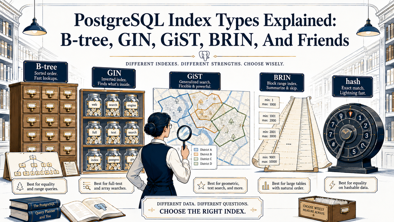
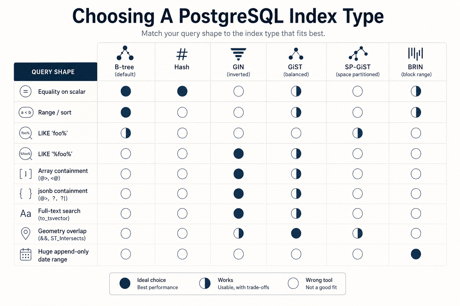
That's because "an index" isn't one thing in Postgres. It's at least six things, each one designed for a very different shape of data and a very different shape of query. And the default, B-tree, is so good at the common case that most of us never bother to learn the rest.

This is a tour of the whole zoo. For each type, we'll go through what it actually does under the hood, when it's the right call, when it's the wrong call, and what an EXPLAIN will look like when it's working. By the end you should be able to look at any column and any query and have an opinion about which index it wants, instead of always reaching for the one Postgres gives you for free.

The mental model: an index is a pre-built lookup structure

Before we get into the types, the one-paragraph version of why any of this matters.

A table without an index is a stack of pages on disk. If you ask "find me the row where email = 'a@b.com'", Postgres has to read every page and check every row. That's a sequential scan, and it's fine for small tables. It's a disaster on a table with 50 million rows.

An index is a separate data structure that maps values to row locations. When you ask the same question, Postgres can walk the index (which is much smaller than the table and laid out for fast lookup) and jump straight to the matching pages. The whole game is "what's the right shape for that data structure?" And the answer depends entirely on what you're searching for.

= on a scalar? Different answer than substring search on text. Different again from "is this point inside this polygon" or "which rows have any of these tags."

That's why Postgres ships several index types. Let's go through them.

B-tree: the default workhorse

A B-tree is a balanced tree where every leaf is the same depth from the root and every node holds a sorted run of values pointing to either deeper nodes or row locations. If you've ever flipped through a phone book, you've used the same algorithm: narrow the range with each comparison.

This is what CREATE INDEX gives you when you don't specify anything:

-- These two are identical
CREATE INDEX users_email_idx ON users (email);
CREATE INDEX users_email_idx ON users USING btree (email);

B-tree is the right answer for the overwhelming majority of cases because it supports the full set of comparison operators: =, <, <=, >, >=, BETWEEN, IN, IS NULL, IS NOT NULL. It also supports LIKE 'foo%', a prefix match, because a sorted tree naturally groups everything starting with foo together. It does not help with LIKE '%foo%' or LIKE '%foo', because there's no way to use a sorted tree when you don't know the start of the string.

It can also satisfy ORDER BY without a sort step. If you have an index on (created_at DESC) and you ask for the 20 newest rows, Postgres walks the leaves in order and stops at 20. That's why pagination on indexed columns feels free and pagination on a ORDER BY some_unindexed_column feels like you're personally aging.

-- Equality, range, prefix, sort — all use B-tree
SELECT * FROM users WHERE email = 'a@b.com';
SELECT * FROM orders WHERE created_at >= now() - interval '7 days';
SELECT * FROM users WHERE email LIKE 'na%';
SELECT * FROM orders ORDER BY created_at DESC LIMIT 20;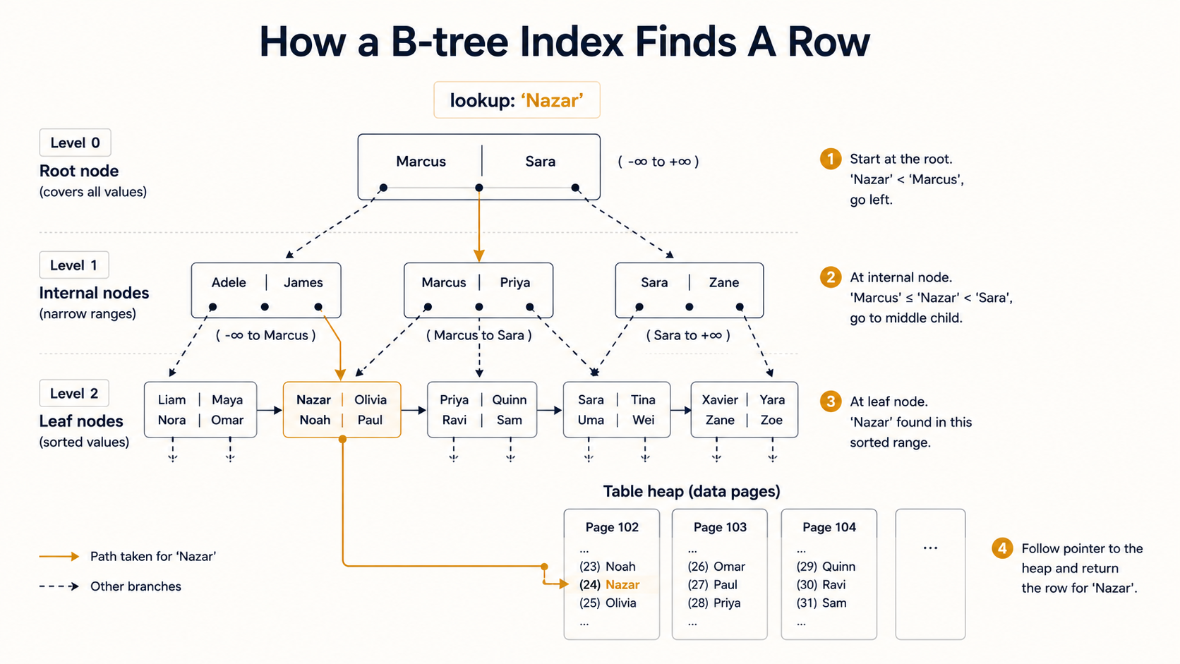

Composite B-tree: column order matters more than you think

You can put multiple columns into one B-tree:

CREATE INDEX orders_user_status_idx ON orders (user_id, status);

This index is great for WHERE user_id = ?. It's also great for WHERE user_id = ? AND status = 'paid'. But it is not great for WHERE status = 'paid' alone, because the tree is sorted by user_id first: finding all rows where status = 'paid' would mean scanning every user_id group. Postgres might still use it if it thinks that's cheaper than a sequential scan, but it won't be a clean lookup.

The rule of thumb: a composite index on (a, b, c) can serve queries on a, on (a, b), and on (a, b, c), but not on b, c, or (b, c) alone. Put the most-filtered column first.

Covering indexes with INCLUDE

Postgres 11 added INCLUDE, which lets you tack extra columns onto a B-tree leaf without making them part of the search key:

CREATE INDEX orders_user_idx ON orders (user_id) INCLUDE (status, total);

Now a query that filters on user_id and only needs status and total can be served entirely from the index; Postgres never has to touch the table. That's an "index-only scan," and it's the fastest type of read Postgres can do. Just be aware: the included columns sit in every leaf, so the index gets bigger.

When B-tree is the wrong tool

B-tree assumes total ordering on the indexed values. That works for numbers, strings, dates, booleans. It does not work well, or at all, for:

• Containment queries on arrays (WHERE tags @> ARRAY['urgent']).
• Substring search inside text (WHERE description ILIKE '%refund%').
• JSON containment (WHERE payload @> '{"status": "open"}').
• Geometric overlap (WHERE polygon && bounding_box).
• Full-text search on tsvector.

For each of those, B-tree either won't get used at all or will degrade into something slower than a sequential scan. That's where the other index types come in.

Hash: the niche specialist

A hash index hashes the value and stores the hash. That's it. It's only useful for =. It can't do range queries, can't do ordering, can't do prefix matching.

CREATE INDEX users_session_token_hash ON sessions USING hash (token);

For a long time, hash indexes had a serious caveat: they weren't WAL-logged, which meant they weren't crash-safe and didn't replicate. That's been fixed since Postgres 10. Today they're real, durable index objects.

But here's the thing: B-tree also handles = perfectly well. So when do you actually want a hash index? In practice, almost never. The case is "you have very long string keys (like UUIDs or session tokens) where the hash is meaningfully smaller than the value, and you only ever do equality lookups." Even then, the difference is small. Most teams just use B-tree and never look back.

I include hash here because it exists, the docs mention it, and you'll see it in interview questions. In real codebases I've seen maybe one in production. You won't be wrong if you skip it.

GIN: for values that contain other values

Here's where things get interesting. GIN (the Generalized Inverted Index) flips the relationship between the indexed value and the row. Instead of "value → row," it stores "element → list of rows that contain this element."

That's exactly what you want when the indexed column is a container. Arrays, jsonb, tsvector, anything where one row holds many things you might search for.

GIN on arrays

CREATE INDEX articles_tags_idx ON articles USING gin (tags);

-- Find articles tagged 'postgres' or 'indexes'
SELECT * FROM articles WHERE tags && ARRAY['postgres', 'indexes'];

-- Find articles tagged with both
SELECT * FROM articles WHERE tags @> ARRAY['postgres', 'indexes'];

Without that index, those queries would scan every row and check the array. With it, Postgres looks up 'postgres' in the inverted index, gets the list of row IDs that contain it, does the same for 'indexes', and combines the results.

GIN on jsonb

CREATE INDEX events_payload_idx ON events USING gin (payload);

-- Find events whose payload contains a specific subdocument
SELECT * FROM events WHERE payload @> '{"type": "checkout"}';

There's also a more selective jsonb_path_ops operator class optimized for containment queries (@>) rather than the full set of jsonb GIN operators and produces a smaller, faster index:

CREATE INDEX events_payload_idx
  ON events
  USING gin (payload jsonb_path_ops);

If you only ever use @> against your jsonb column (which is the common case for "does this event match this filter"), jsonb_path_ops is almost always the right call.

GIN for full-text search

CREATE INDEX articles_search_idx
  ON articles
  USING gin (to_tsvector('english', body));

SELECT * FROM articles
WHERE to_tsvector('english', body) @@ plainto_tsquery('english', 'index types');

GIN is the standard choice for tsvector because lookups dominate writes in most search workloads, and GIN gives you faster reads than GiST at the cost of slower writes.

When GIN is the wrong tool

GIN's reads are fast and its writes are slow. Each insert or update has to walk the indexed value, decompose it into elements, and update potentially many leaves. There's a "fastupdate" mechanism that batches writes into a pending list and flushes them in chunks, which helps for bursts but adds latency to occasional reads when the flush is triggered mid-query.

If your table is write-heavy and the column being indexed has lots of elements per row, GIN can become a bottleneck. Measure before you commit.

GiST: the generalist

GiST (the Generalized Search Tree) is less an index and more a framework for building indexes. It gives extension authors a way to say "here's how to compare two values, here's how to split a node when it gets full," and Postgres handles the tree mechanics.

That's why GiST shows up in so many different places: PostGIS for geometry, pg_trgm for trigram-based fuzzy search, range types, exclusion constraints. They're all GiST under the hood, with different operator classes plugged in.

GiST for ranges

CREATE INDEX bookings_period_idx ON bookings USING gist (period);

-- Find bookings overlapping a given range
SELECT * FROM bookings WHERE period && tstzrange('2026-06-01', '2026-06-08');

A B-tree can't help with range overlap because there's no total ordering on ranges. GiST handles it natively.

This also enables one of Postgres's underrated tricks: exclusion constraints.

CREATE TABLE bookings (
  room_id   int,
  period    tstzrange,
  EXCLUDE USING gist (room_id WITH =, period WITH &&)
);

That single constraint says "no two bookings for the same room can have overlapping periods." The database enforces it. You don't have to write the check in application code, you don't have to wrap inserts in a transaction with a manual lock; the index does it.

GiST for fuzzy text with pg_trgm

This one is genuinely useful. The pg_trgm extension splits text into 3-character trigrams and indexes them, which lets you do similarity search and substring matches:

CREATE EXTENSION IF NOT EXISTS pg_trgm;

CREATE INDEX users_name_trgm_idx
  ON users
  USING gist (name gist_trgm_ops);

-- Substring match — works because of the trigram index
SELECT * FROM users WHERE name ILIKE '%marcus%';

-- Similarity match — finds typos
SELECT * FROM users WHERE name % 'markus';

This is the answer to "how do I make LIKE '%foo%' fast." You can't with B-tree. You can with a GiST or GIN index over trigrams.

For trigram search, GIN is usually faster for read-heavy workloads (USING gin (name gin_trgm_ops)), GiST for write-heavy or when you need ORDER BY similarity. Try both. Their performance profiles cross over depending on the data.

When GiST is the wrong tool

GiST's structure means lookups can require visiting multiple branches; the comparison function decides which branches might contain a match, and "might" is doing a lot of work. For exact-match queries on simple types, B-tree is faster. Use GiST when you actually need its flexibility: ranges, geometry, fuzzy text. Don't reach for it because it sounds general-purpose.

SP-GiST: for data that doesn't balance

SP-GiST (Space-Partitioned GiST) is for data structures that are inherently unbalanced. Think quadtrees, kd-trees, suffix trees, radix trees. The key distinction from GiST is that SP-GiST partitions the search space into non-overlapping regions, while GiST allows overlap.

That sounds abstract. The practical case: indexing data that has natural hierarchical clusters where some clusters are dense and others are sparse, like phone numbers (most start with a few common area codes), or IP addresses (most live in a few prefixes), or text strings (most share leading characters).

-- Radix-tree index on text (good for prefix searches)
CREATE INDEX users_email_spgist_idx
  ON users
  USING spgist (email);

-- Quadtree index on points
CREATE INDEX places_location_idx
  ON places
  USING spgist (location);

In honest practice, you'll rarely reach for SP-GiST yourself. It's mostly used by extensions and by Postgres internally for specific data types. If you've never used it, you're not missing much. If you have a workload with very skewed key distribution and B-tree is performing poorly, it's worth knowing this exists.

BRIN: for huge tables with naturally-ordered data

BRIN (Block Range Index) is the index type that earns its keep when your table is enormous and the data has natural physical ordering on disk. Append-only logs, time-series data, audit trails: these tables grow forever, and the rows are written in roughly the order you'll later query them.

A BRIN index doesn't store one entry per row. It stores summary info (typically min and max) for a range of pages. By default, one summary per 128 pages. So a 100 GB table with default settings produces a BRIN index measured in megabytes, not gigabytes.

CREATE INDEX events_created_at_brin_idx
  ON events
  USING brin (created_at);

SELECT * FROM events
WHERE created_at >= '2026-05-01'
  AND created_at <  '2026-05-02';

When the query asks for a date range, Postgres scans the BRIN index, finds the page ranges whose summaries overlap the requested range, and reads only those pages from the table. Compared to a full table scan, you might read 0.1% of the pages. Compared to a B-tree, you got the same effect with an index that's a thousand times smaller.

The catch

BRIN only works well when the column you're indexing correlates strongly with physical row order. If created_at was always written in increasing order (true for most append-only tables), every row written on May 3rd lives in a small contiguous run of pages, and BRIN's summaries are tight. The index points you straight to the right slice of the table.

If you indexed something like user_id instead (where row 1 might belong to user 4, row 2 to user 9012, row 3 to user 17), every page range covers the entire range of user IDs, and the BRIN index becomes useless. The summaries say "this page might contain any user," because it might.

You can check the correlation Postgres has measured:

SELECT attname, correlation
FROM pg_stats
WHERE tablename = 'events';

A correlation close to 1 (or -1) means tightly ordered. Close to 0 means BRIN won't help.

You can also tune the page-range size with pages_per_range if your access pattern queries narrower ranges than the default 128 pages handles well:

CREATE INDEX events_created_at_brin_idx
  ON events
  USING brin (created_at) WITH (pages_per_range = 32);

Smaller ranges → bigger index, more selective lookups. Larger ranges → smaller index, more pages read per query. The right value depends entirely on your query shape.

Bloom: the multi-column equality trick

Bloom is an extension, not a built-in. You enable it with CREATE EXTENSION bloom;. It's worth a paragraph because it solves a specific problem the others can't.

Imagine a table with a dozen columns, and your queries filter on different combinations of any three of them at a time. A B-tree per column might or might not get used, depending on selectivity. A composite B-tree per combination would mean dozens of indexes. Bloom indexes are small probabilistic structures that can give you "this row probably matches" for any combination of columns, then Postgres re-checks the actual values:

CREATE EXTENSION IF NOT EXISTS bloom;

CREATE INDEX wide_table_bloom_idx
  ON wide_table
  USING bloom (a, b, c, d, e, f, g);

It's niche. The typical case is data warehouses with many low-cardinality columns where users filter on different subsets. For OLTP, you almost never want this.

Three modifiers that work with most index types

These aren't index types; they're modifiers you can apply to (mostly) any index type. They don't get the attention they deserve.

Partial indexes: index only the rows you query

CREATE INDEX active_users_email_idx
  ON users (email)
  WHERE deleted_at IS NULL;

If 90% of your users rows are deleted but you only ever query the active ones, this index is a tenth the size of a full one and faster to walk. Postgres uses it whenever your query's WHERE clause implies the same predicate.

-- Uses the partial index
SELECT * FROM users WHERE email = 'a@b.com' AND deleted_at IS NULL;

-- Does NOT use the partial index — Postgres can't prove the row matches the predicate
SELECT * FROM users WHERE email = 'a@b.com';

This is one of the most underused features in Postgres. Status flags, soft-delete tombstones, completed/in-progress markers: all great candidates.

Expression indexes: index the result of a function

CREATE INDEX users_lower_email_idx ON users (lower(email));

-- Uses the index
SELECT * FROM users WHERE lower(email) = 'a@b.com';

Without that index, the function call on every row would force a sequential scan. With it, Postgres pre-computes lower(email) for every row at write time and indexes the result. The function must be IMMUTABLE for this to work.

Combine it with pg_trgm and you've got case-insensitive fuzzy search:

CREATE INDEX users_lower_email_trgm_idx
  ON users
  USING gin (lower(email) gin_trgm_ops);

Covering indexes with INCLUDE

Already mentioned under B-tree, but worth repeating: INCLUDE lets you bolt extra columns onto an index so reads can be served entirely from the index without touching the table. Watch the index size; every included column ships with every leaf entry.

How to know which one is being used

Whatever index you create, the only way to know it's actually getting used is EXPLAIN:

EXPLAIN (ANALYZE, BUFFERS)
SELECT * FROM users WHERE email = 'a@b.com';

Look for the access method:

• Seq Scan: no index used, full table scan.
• Index Scan using <index_name>: index used, then heap visited for full row data.
• Index Only Scan: index alone served the query (great for INCLUDE setups).
• Bitmap Index Scan + Bitmap Heap Scan: Postgres collected matching row IDs from the index, sorted them, then read pages in order. Common for medium-selectivity queries and for combining multiple indexes.

If you see Seq Scan on a query you expected to use an index, the usual suspects are: data type mismatch (WHERE id = '42' against an int column), function call on the column (WHERE date(created_at) = ... instead of a range), low selectivity (the planner thinks reading the whole table is cheaper), or a missing or invalid index. BUFFERS tells you how many pages were actually read, which is the truest measure of whether your index is helping.

A quick decision guide

Skipping the templated "Final Tips". The article isn't a checklist. But if you want one paragraph to take with you: B-tree is right for almost everything. Reach for GIN when the column contains many things (arrays, jsonb, tsvector). Reach for GiST when you need overlap, range queries, or fuzzy text. Reach for BRIN when the table is huge and the column correlates with physical order. Hash exists, but you can probably ignore it. SP-GiST and Bloom are real but rare; you'll know when you need them.

The pattern that holds for all of them: the right index isn't the one that sounds most powerful. It's the one whose structure matches the shape of the query you actually run.